Hansard Text Analysis (Part 2)
This article will explore how text mining can be used to gather data from Parliamentary transcripts (Hansards) using the R programming language and tidy data principles. I focus specifically on a Hansard from the House of Lords regarding the EU withdrawal bill which can be found here. This will build on ideas from another article I wrote: if you haven’t read the first part, find that here. I will again lean heavily on methods I learned from Julia Silge and David Robinson in their book Text mining with R and the tidytext package. Be sure to use the Parliament website glossary for tricky phrases.
What does text-mining analysis look like? Usually we have a set of related documents (e.g. news articles about different businesses) known as a corpus. Often, these articles don’t come in a format immediately appropriate for analysis so will first have to be “cleaned” and “standardised”, but we will ignore that for now. Every text mining analysis then seeks to convert features of the text into numerical values. This is just a fancy way of saying: first, we need to count things.
But what’s our goal here? What information can we “mine” from the text that you can’t get from just reading it? The first goal is summarisation. We can condense information down and extract the most important parts in a way that can be easily scaled. The second goal is clarification. When you read a debate, you have certain intuitions and feelings about what went on. “Those three spoke about similar things”. “He was the most aggressive”. We want to quantify these things, and by putting numbers on them make statements in a statistically rigorous, evidence-based way. We can make unbiased searches for every pattern in the text, even ones that people might miss after a few readings. The third goal for lots of text mining work is prediction. You have gathered information on what is there, and maybe you can use this again in the future to predict something in another text. This is a bit beyond the scope of this article, but an example might be using the data you have gathered from one set of speeches to predict the party of a speaker in a new speech.
The approaches used here are useful for another simple reason: automation. Letting a program collect some of the available data for us is much faster and more accurate than doing things by hand.
Let’s start with what we can count. This will act as an outline for the rest of the article:
- Total number of words (per speech)
- Number of individual words
- Number of other grammatical features of the text (punctuation, grammatical category)
Another thing to consider is that the Hansard has a temporal element, meaning we can order the speeches chronologically. We might also be able to use some tricks to investigate how words are used in the context of other words (counting pairs/multiples of words, correlations of words between speeches, graph-based methods, etc…).
Speech lengths
We’ll start with the simplest detail relating to the words in our Hansard- how many are used in total each speech.
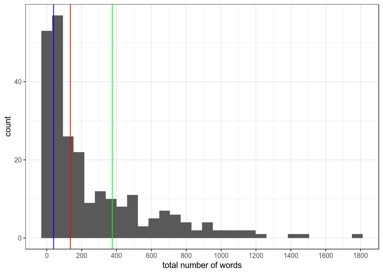
Figure 1: Distribution of speech lengths with vertical bars for lower quartile, median and upper quartile.
The vast majority of speeches were at the shorter end of the distribution. The median number of words used was 135, with 75% of speeches using less than 418 words. The top 25% of speeches in terms of word counts range from 418 to almost 1800.
For comparison, take a look at Baroness Smith’s 135 word speech here and Baroness Stowell’s 420 word speech here for comparison.. Using my internal “speech length” indicator, these results are telling me that 75% of speeches are not really very long at all. Indeed, a 400 word speech only takes 1.5 to 2 minutes to read aloud.
We also know that different MPs used different numbers of speeches. We would expect to see that the more speeches you make, the more words you use. Is this the case?
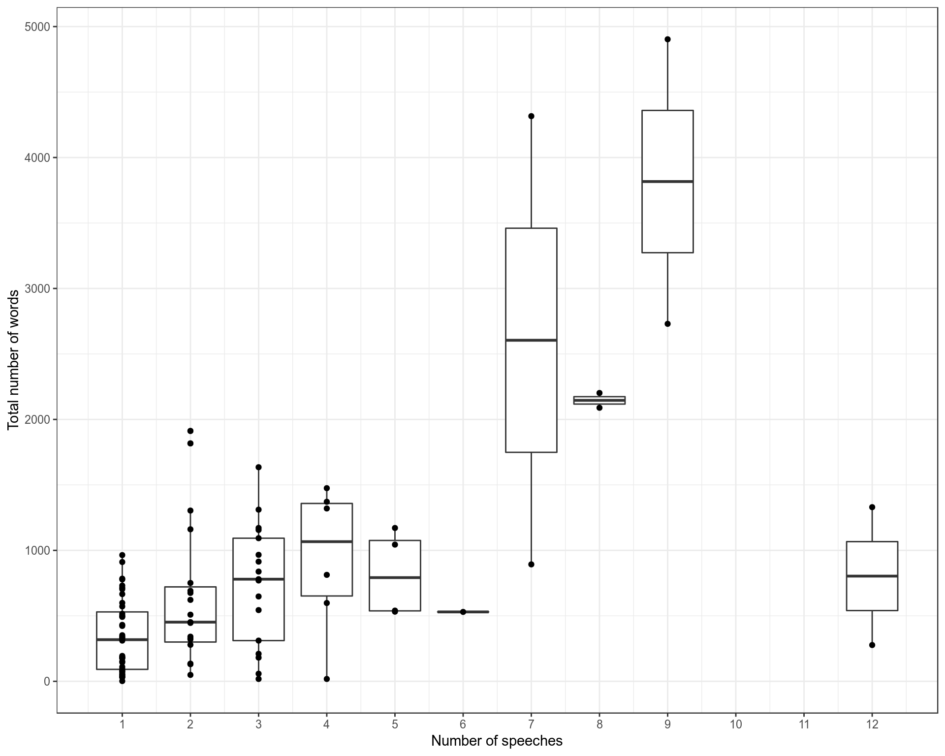
Figure 2: The relationship between the number of speeches a lord gives and the number of words they use.
As we might expect, the more speeches you give, the more words you use in total. But this correlation is far from perfect and there is a glaring outlier in the two Lords who made 12 speeches both using hardly any words.
Let’s pick out the peers who made five or more speeches, and look not just at the total number of words, but the number of words used in each of their speeches (to understand the spread).
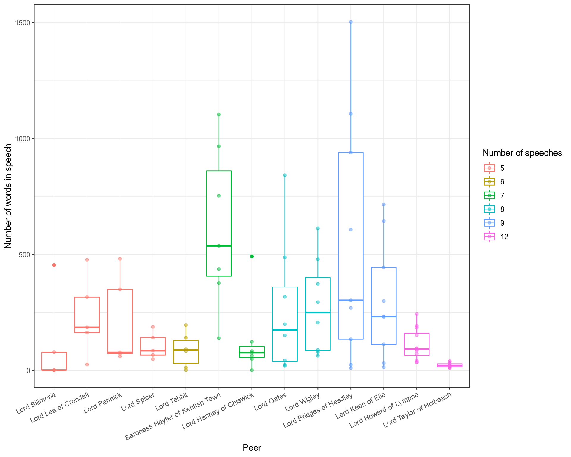
Figure 3: As above but with specific boxplots for each peer.
There are clearly different strategies, or perhaps roles, for each different MP. Baroness Hayter makes a similar number of speeches to Tebbit and Hannay, but her speeches are generally longer (none being exceptionally short or long). Lord Taylor, in contrast has an incredibly tight distribution of very short speeches. This is telling- he is in fact the whip of the Conservative party, so his speeches consist exclusively of short rebukes. Lord Howard, a eurosceptic, speaks as a contrarian to many of the amendments moved by other MPs, leading to a large number of short arguments. Lord Bridges, who shows the most variation in speech lengths, was the Government’s secretary for DxEU.
As we can see, even these raw numbers of words tell a story. But now we will move onto…
The text itself.
Boring definitions: Each text is composed of words. People who research text mining and apply this in natural language processing (NLP) refer to each body of text as a document. Think different newspaper articles, different books by an author. We could treat all of these as documents. Corpus is the word used to refer to a collection of documents. Now let’s think about scale. There are lots of Hansards about Brexit. So we could (and later will) make a corpus of Hansard documents. But here, I have chosen to focus on what can be gleaned from a single debate. For our purposes, we will treat speeches as each document, and the corpus will be the collection of speeches in the Hansard.
Figure 4: Word counts, n (with stop words removed)
The first thing we do is count the number of times each word occurs in each speech, and also the total number of words in each speech. Unsurprisingly in a bill about Britain’s withdrawal from the EU, terms like “EU”, “citizen” and “European” come up often. So does “Lord”, which is also unsurpising given the location of the debate. But we also see words like “women”, “nuclear”, “euratom” (the European Atomic Energy Community) and “devolved” being used many times in some speeches. Is there a better way for us to access this information about which words were most important in the debate?
Calculating the importance of words
What words are most important in each speech? How can we rank words in terms of importance? Simple questions. Difficult to answer. We’ll go through some examples to understand why defining which words are important to a speech is difficult, and how to get around these problems. But first, here is one way researchers calculate the importance of a word: TF-IDF (Term frequency-Inverse document frequency).
TF-IDF = Term Frequency * Inverse Document Frequency
In our case, this means
TF = (Number of times term appears in speech) / (Total number of terms in the speech) IDF = log_e(Total number of speeches / Number of speeches with term in it)
I explain TF-IDF in detail below, so if you already know what TF-IDF means feel free to skip this bit. If you want a really short and sweet explanation of TF-IDF go to http://www.tfidf.com/.
Question
What if we just find the most common words? Surely the words that appear most are the most important?
Challenge
The most common words are just going to be uninformative ones like “the”, “and”, etc…
Solution
After counting the frequency of each word in a speech, we can remove stop words. This is literally an arbitrary list of “common” words which we have decided not to include in the analysis and remove. It’s not flashy, but it’s useful for what we’re doing here and is how I got counts in the table above.
Counting the frequency of words gives us what researchers call the “term frequency” for a document.
Question
Now we have counts of informative words, aren’t the most common ones the most important?
Challenge
Maybe. Earlier in the article we showed that speeches are of different lengths. A word which is used 50 times must be important, you might say? What if this was in a 50,000 word document? Probably not so important.
Solution
We divide the frequency of each word by the total number of words in that speech. If we didn’t normalise like this, when we try to compare the most important words between speeches, words from longer speeches would end up outranking words from shorter ones, even though they might proportionally have been used less.
Question
We’ve calculated the “normalised term frequency”. What on earth else is needed to tell us what the important words are?
Challenge
What do we actually mean by important? Imagine you have a set of newspapers articles about education. The word “school” and “teacher” probably appears in every document (with varying frequency), so we could penalise these words allowing other words that distinguish different speeches to be found. We could just remove these words that are shared between documents (treat them as “stop words”). But there is a better solution.
Solution
When we have our term frequency, we can multiply this by the “Inverse document frequency” for that word. How do we calculate this? Say you have 10 documents. You’re word appears in 8 of them (it’s a pretty common word). The inverse document frequency is equal to log(10/8). Let’s compare how this changes if we make our word rarer amongst the documents.
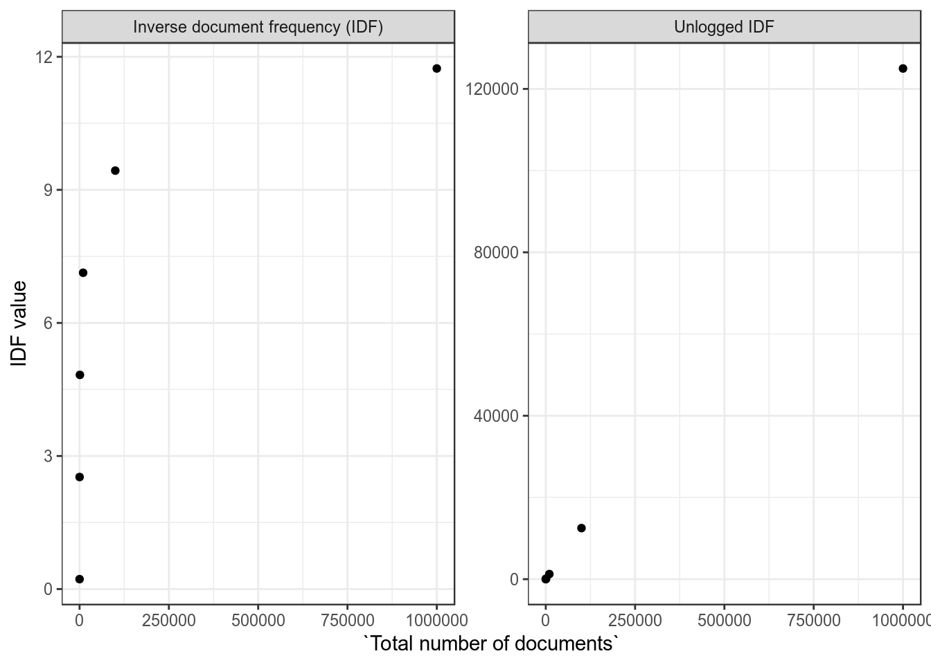
Figure 5: If a word appears in 8 documents, how does the IDF change as we increase the number of documents?
The unlogged IDF shown for comparison. We just log the value so that this “IDF multiplier” stays within a reasonable range- the IDF increases in a linear way as the number of documents increases by orders of magnitude.
That aside, as documents containing our word become rarer, the word’s IDF score increases. This is the important thing. Think about what this means:
TF-IDF (“Word importance”) = Term frequency * Inverse Document Frequency
More frequent terms get a higher score (good). Words that appear in a smaller fraction of documents get a higher score (also good). So if a word is unique to a speech and is used in it often, it gets a high score, because it defines that speech and not others. Low scoring words are either not used a lot in any speeches, or appear in almost every document- meaning they can’t be used to accurately define any of them.
TF-IDF for the longest speeches
Let’s take the six longest speeches, and which words were picked out as the most important ones.
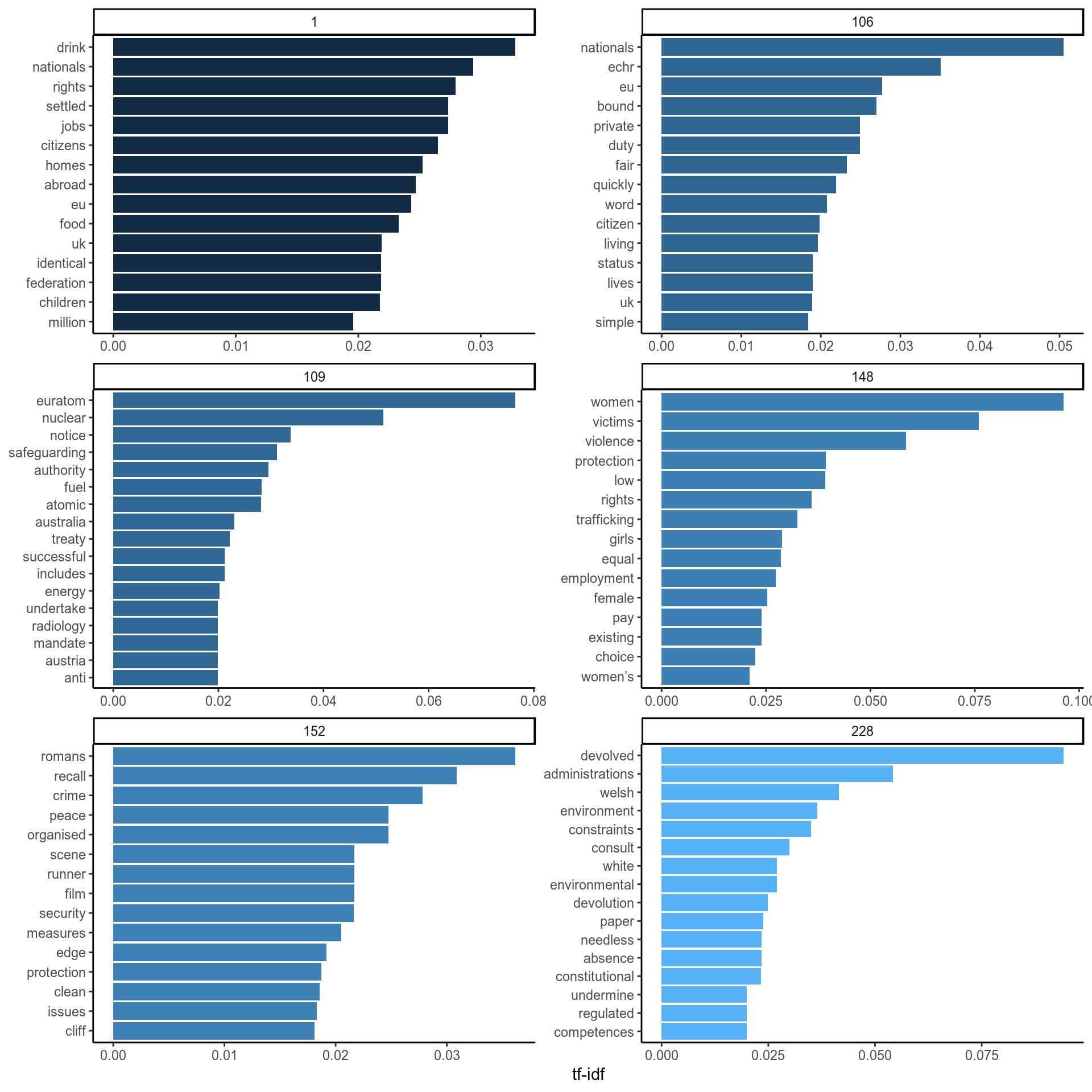
Figure 6: The words are on the y axis and their TF-IDF is the position of each bar on the x axis. Each panel is a different speech.
Looks messy, let’s talk it through. Generally, TF-IDF seems to have pulled out words that are important in these speeches ranked in the top 10. There are also words that are important but won’t make sense without further context (speech 1 has it’s top word as “drink” because the peer mentions the “food and drink federation” repeatedly). Other words seem to not have the “right” rank if we were to do it ourselves intuitively. Finally, there are words with a high TF-IDF that aren’t representative of the speech at all (“romans” doesn’t really tell us anything about speech 152). But in general, we can see that speech 148 is about womens rights, 109 about Euratom and nuclear safety and 228 about the role of devolved administrations. 1 and 106 are less clear but seem to be about fair rights for EU nationals and UK citizens. Speech 152 seems a bit unclear and no one word has a particularly high TF-IDF anyway.
As a complete and inconsequential aside before we move on, here are the top 10 TF-IDF scores from every speech in rank order from most important to least important.
I’ll put it down to the absurdity of the universe that “bullet”, “minorities” and “bodies” appeared as the top three most important words, and try not to worry too much about it.
Hansard timeline using TF-IDF
We are going to use TF-IDF as a way to summarise the Hansard. We have seen how this is like pulling important words from a “bag of words” (each speech). The meaning from the context which the words were used in is inevitably lost, but it’s a useful heuristic and the way TF-IDF is calculated is transparent (not a black box).
Below is a pretty cool graphic (Open it in a new tab!), where I’ve extracted the word with the largest TF-IDF from each speech longer than 50 (non-stop-word) words and displayed them chronologically. The size of the word represents its TF-IDF.
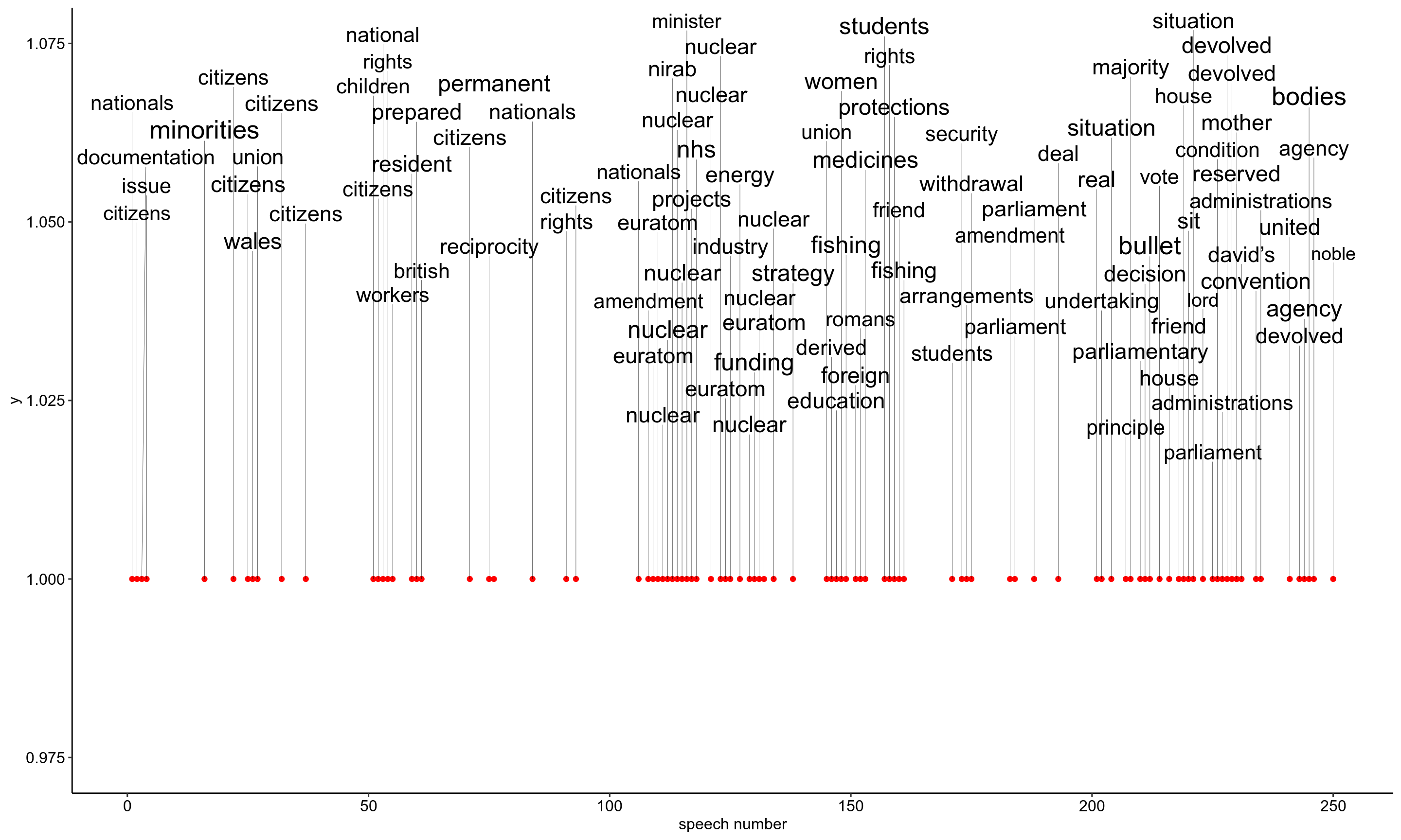
Figure 7: The position of words on the y axis is irrelevant! Cheers to Kamil Slowikowski (https://slowkow.com/) for making ggrepel which organises the text so nicely.
Early on in the debate, there’s lots of talk about “citizens”. Then there is a period of debate about nuclear bodies/Euratom. Then a period where lots of industries and issues are mentioned including education, fishing, the NHS and women’s rights. The rest of the debate is largely about Parliamant’s role in the decisions made by the government, and the assurances for devolved administrations.
So TF-IDF is a pretty cool method for finding out the most important words in a text. But what are some problems with it? You might already have noticed some.
- If a word in few documents is used often in a text -even if it does not represent the text at all- it will be promoted to the highest TF-IDF (look at “Romans” above).
- In light of this idea of “representativeness” of the high scoring words, TF-IDF is what we call a bag of words method for analysing text. We have just taken all the words and counted them. In doing this, we ignore the context which words are used in. We ignore the semantics of the sentence. A more nuanced summary is difficult to achieve using TF-IDF alone.
- Shorter texts suffer from the fact that no ‘interesting’ words occur frequently, so we’re more likely to get unrepresentative words scoring high TF-IDFs. Similarly, how much do we trust a word with a term frequency of 2 which has scored highly because the text was short and it occured in very few documents?
Conclusions
In this article, we have explored how simply counting the number of words in speeches can reveal things about a Hansard. We talked in detail about how we can use these counts to create a useful scoring system (TF-IDF) for finding important words in documents, culminating in a summarised timeline of topics discussed in the Hansard. We also talked about the limitations of this method. What did we find out about Britain’s withdrawal from the EU based on this Hansard? Figures 2 and 3 told us something about how we can think about the contribution of different Lords to the debate by looking at the number of speeches they make and the number of words they use. We then saw how TF-IDF can be used to distinguish important words for each speaker. Common themes for this debate appeared to be nuclear energy, the ‘trade-off’ of rights of EU citizens and British nationals, the future roles of devolved administrations, and what Parliament’s role is in all this.
But this is barely scratching the surface of what can be achieved using text mining. More advanced methods are available, and the amount you can learn using simpler techniques can often be extended if you apply them more creatively. Next time we will discuss how ideas like bigrams, regular expressions searches, sentiment analysis, latent dirichlet allocation and more can be used to glean information from the Hansard. Here is a link to the github page for this project if you’d like to look at the code. Please send feedback to mchaib[dot]blog[at]gmail[dot]com.